Día 22: El norte no siempre está arriba
Este debería ser el mapa en 5 minutos pero es el norte no siempre está arriba versión poco esfuerzo. En vez de graficar la anomalía de la altura geopotencial alrededor del polo sur, hoy es alrededor del polo norte!
sf::sf_use_s2(FALSE)
mapa <- rnaturalearth::ne_coastline(returnclass = "sf") %>%
  sf::st_crop(xmin = -180, xmax = 180, ymin = 5, ymax = 90)

z <- ReadNetCDF("datos/geopotencial_era5.nc")

grid <- expand.grid(longitude = seq(0, 360, by = 2.5),
                    latitude = seq(-90, 90, by = 2.5))

z %>%
  .[level == 200] %>%
  .[latitude > 0] %>%
  .[, gh.z := Anomaly(z), by = .(latitude)] %>%
  .[, c("u", "v") := GeostrophicWind(gh.z, longitude, latitude)] %>%
  .[grid, on = .NATURAL] %>%
  na.omit() %>%
  ggplot(aes(longitude, latitude)) +
  geom_contour_fill(aes(z = gh.z,), xwrap = c(0, 360), breaks = seq(-3000, 2000, 500)) +
  geom_contour_tanaka(aes(z = gh.z), xwrap = c(0, 360)) +
  geom_sf(data = mapa, inherit.aes = FALSE, linewidth = 0.3) +
  # geom_streamline(aes(dx = dlon(u, latitude), dy = dlat(v)),
  #                 dt = 100, S = 100,
  #                 xwrap = c(0, 360), arrow = NULL) +
  scale_fill_divergent(guide = guide_colorsteps(barwidth = 0.5,
                                                barheight = 15),
                       breaks = seq(-3000, 2000, 500)) +
  coord_sf(crs = "+proj=laea +lat_0=90", default_crs = "+proj=lonlat", lims_method = "orthogonal") +
  labs(x = NULL, y = NULL, fill = NULL,
       title = "Anomalía de la altura geopotencial en 200 hPa y viento geostrófico",
       subtitle = "Promedio mensual para octubre de 2023",
       caption = "Fuente: ERA5 - Reanalisis Europeo") +
  theme_void(base_size = 10,
             base_family = "Roboto Condensed Light") +
  theme(plot.title = element_text(face = "bold"),
        plot.margin = unit(c(0.3, 0.3, 0.3, 0.3), "cm"))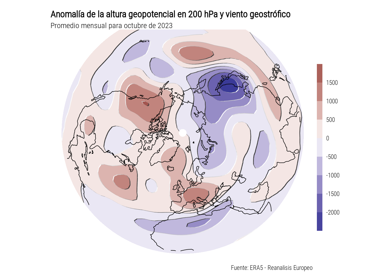
ggsave("day22.png", device = png, type = "cairo", bg = "white", width = 14, height = 13, units = "cm", dpi = 150)